What is Optimization? - Solving LinkedIn Games by Linear Optimization

The mathematical optimization process consists of modeling a problem with the goal of minimizing (or maximizing) a function, e.g., minimizing the total cost of a transportation system (or maximizing the expected total profit of a project). Mathematical optimization modeling fundamentally involves formulating the objective function $f(\mathbf{x})$ that one seeks to optimize, and a set of constraints that translates the limitations, specifications, assumptions and rules a problem may present and delimits the feasible set $D$ of solutions to the problem. Thus, the most general and abstract formulation for an optimization model is as follows.

\text{Min} \ f(\mathbf{x})

\begin{array}{rl} \text{S.t.:} & \\ & \mathbf{x} \in D \\ \end{array}

The vector $\mathbf{x} = [x_1, x_2, \cdots, x_i]$ corresponds to the vector of decision variables for the problem, whose solution $\mathbf{x}^*$ represents the optimal solution of the problem, that is, the set of values that minimize or maximize the objective function.

To better illustrate how the application of an optimization model works, let’s consider the following example:

The terrain in the presented situation can be represented on a Cartesian plane $xy$ , where the point $(0,0)$ corresponds to the center of the base of the semicircle and the boundaries of the terrain are given by the region $D = \{(x, y) \in \R^2 \mid x^2 + y^2 \le r^2, y \ge 0\}$ (where $r$ is the radius of the semicircle), which corresponds to the feasible region. Since the problem seeks to maximize the area of the terrain, it is assumed that the vertex where the walls should meet is located on the semicircle, and the question boils down to finding the $x$ and $y$ positions of the vertex that maximize the area $A$ of the construction. Since the base $w$ of the building is $2x$ and its height $h$ will be given by the value of the $y$ coordinate, then the area of the construction will be given by the objective function $A(x,y) = 2xy$ . Given all the specifications, the model used to solve this exercise will be given by:

\text{Max} \ A(x,y) = 2xy

\begin{array}{rl} \text{S.t.:} & \\ & x^2 + y^2 \le r^2 \\ & x \ge 0 \\ & y \ge 0 \\ \end{array}

From this model, it is possible to discover, by applying the KKT Conditions (see more on Appendix), that the pair $(x, y)$ that maximizes the building’s area and satisfies the specified constraints is given by $(x^*, y^*) = (\frac{\sqrt{2}}{2}r, \frac{\sqrt{2}}{2}r)$ , which results in the optimal plot of $A(x^*,y^*)=\frac{r^2}{2}$ . Since $r = 10$ , the optimal dimensions are $(w^*, h^*) = (10\sqrt{2}, 5\sqrt{2})$ and the optimal area $A^*$ is 50 m².

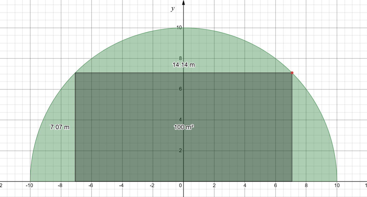
Semicircular Terrain's Solution — Figure 2:The dimensions $(w^*, h^*) = (10\sqrt{2}, 5\sqrt{2})$ result on a optimal area of $A^*=50$ m². *Figure made on Desmos*

Components of an Optimization Model¶

Every optimization model is built from a set of components that together define the problem to be solved. These components describe the universe of values, the choices we can make, the constants we cannot change, and the rules that those choices must obey. When these components are combined, an optimization model becomes a precise mathematical description of a decision problem. The solver then searches for the decision variable values that satisfy all constraints and optimize the objective function. The main components of an optimization model are:

Ranges: They are the basic domains used to define the indexes for other components. They tell the model which values are valid for a given index and are typically written as ordered sequences or sets, such as the rows of a matrix, the columns of a board, or the time periods in a schedule. E.g., if my problem involves a set of distribution centers and a set of customers, I might define a range for the distribution centers as $I = \{1, 2, 3\}$ and a range for the customers as $J = \{1, 2, 3, 4\}$ . These ranges allow us to write constraints and objective functions that refer to all distribution centers or all customers without having to list them individually, which allows for more compact and general formulations.
Sets: They are collections of related elements built from ranges or defined explicitly. E.g. if a problem deals with a range of suppliers and a range of customers, I might define a set of possible routes between them as $R = \{(i,j) \mid i \in I, j \in J\}$ , which represents all possible relations or routes between suppliers and customers. Well defining sets make it easier to write constraints over many elements without listing them one by one.
Decision Variables: They are the unknowns the model is trying to determine. They represent the choices available to the decision-maker, such as the decision to buy or not buy a certain item, how long to keep a machine running, or how much of an item to produce. In mathematical notation, decision variables are typically written as $x_i$ , $x_{ij}$ , or $x_{ijk}$ , and they can be continuous, integer, or binary depending on the problem.
Parameters: They are the fixed values that describe the problem data. They do not change during optimization and are used to define costs, capacities, pre-filled values or other constants. Examples include the cost of a route, the size of a board or the fact that a specific square is pre-filled in a puzzle.
Objective Function: It’s the formula that the model seeks to minimize or maximize. It is expressed in terms of the decision variables and parameters, and it captures what we care most about in the problem. Common examples include minimizing total cost, maximizing coverage, or maximizing the number of correctly placed pieces. The objective function gives the model a direction and a single numerical criterion for choosing the best solution.
Constraints: They are the rules that the decision variables must satisfy. They define the feasible region of the model and ensure that the solution obeys the problem’s physical, logical, or specific requirements and premisses. E.g., in the context of a transportation problem, constraints can require that the total amount shipped from a supplier does not exceed its capacity, or that the total amount received by a customer meets its demand. Also, they might define basic restrictions such as non-negativity of decision variables, or that a certain variable must be binary (0 or 1) or an integer.

Linear Optimization¶

Linear Optimization (LO), or Linear Programming, works with a subset of optimization problems in which both objective function and set of constraints are linear formulas, that is, written as a sum of products between constants and variables, as in the following example.

\text{Min} \ a_1 x_1 + a_2 x_2 + \cdots + a_n x_n

\begin{array}{rll} \text{S.t.:} & \\ & a_1 x_1 + a_2 x_2 + \cdots + a_n x_n = c_i, & \forall i \in I \\ & a_1 x_1 + a_2 x_2 + \cdots + a_n x_n \le k_j & \forall j \in J \\ & x \ge 0 \end{array}

This kind of model represents a Linear Optimization Problem (LOP). If the objective function is not linear or the problem has at least one non-linear constraint, then it’s a Non-Linear Optimization Problem (NLOP) and one should need Non-Linear Programming (NLP) techniques to solve it.

Linear Optimization Hypotheses¶

Because the objective function and the model constraints are linear expressions, an LOP implicitly assumes at least four hypotheses in its modeling:

Proportionality: The contribution of each decision variable to the objective function and to the model constraints must be directly proportional to its value. Situations that take into account economies of scale, initial manufacturing setup costs, etc., are examples where this principle is violated.
Additivity: The contribution of each decision variable to the objective function and to the model constraints must be directly proportional to its value. Situations that take into account economies of scale, initial manufacturing setup costs, etc., are examples where this principle is violated.
Divisibility and non-negativity: Each of the decision variables can take any values within the set of positive real numbers, as long as they satisfy the model’s constraints.
Certainty: The coefficients and independent terms of the objective function and the model’s constraints are deterministic, that is, if it is modeled that $z(x,y)=2x+3y$ , it would be assumed that the coefficients 2 and 3 of $x$ and $y$ , respectively, would be known and certain, that is, it would be certain that the contribution of $x$ to $z$ would always be 2 times the amount of $x$ , while the contribution of $y$ to $z$ would always be 3 times the amount of $y$ , no matter what the values of $x$ and $y$ are. In the BLOP model for the Queens game, all coefficients and independent terms will be equal to 1 (except for the arbitrary constant $C$ , which can take any value, as will be seen later).

Why Python?¶

Python is a high-level, interpreted programming language that is widely used in the field of optimization due to its simplicity, readability, and extensive library support. It provides a rich ecosystem of packages for mathematical computing, data analysis, and machine learning, making it an ideal choice for implementing and solving optimization models. Python’s syntax is straightforward and easy to learn, which allows practitioners to focus on the logic of their optimization problems rather than on complex programming details. Additionally, Python has powerful libraries such as NumPy for numerical computations, Pandas for data manipulation, and Matplotlib for visualization, which can be very helpful in analyzing and interpreting optimization results. Moreover, Python interfaces with many optimization solvers, making it a versatile tool for both academic research and industry applications in optimization.

Why not use Excel Solver, OpenSolver or other optimization software?

While Excel Solver and other optimization software can be useful for solving simple optimization problems, they have limitations that may not be suitable for more complex or large-scale problems. Excel Solver, for example, has a native limit of 200 decision variables and 100 constraints it can handle, which can be a significant drawback for larger optimization problems. On the other hand, Python provides a more flexible and powerful environment for modeling and solving optimization problems, with access to a wide range of libraries and solvers that can handle various types of optimization problems efficiently.

Furthermore, modelling on a spreadsheet can become cumbersome and error-prone as the complexity of the problem increases, while Python allows for more structured and modular code, making it easier to manage and debug. For example, if a problem have hundreds of decision variables and constraints, it would be difficult to keep track of all the formulas and references among cells, while in Python you can create all the components with just a few code lines, which makes the reasing more clear and readable.

Additionally, Python’s ability to integrate with data analysis and visualization tools allows for better interpretation and communication of optimization results, which can be crucial for decision-making processes. Therefore, while Excel Solver can be a convenient tool for simple problems, Python is often the preferred choice for more complex optimization tasks due to its flexibility, scalability, and powerful libraries.

Python Libraries¶

Along this book, it’ll be used the following Python libraries:

Pyomo: A powerful and flexible optimization modeling language that allows users to define optimization problems in a clear and concise way. Pyomo supports a wide range of optimization problem types, including linear, integer, and nonlinear programming, and can interface with various solvers.
NetworkX: A library for the creation, manipulation, and study of complex networks. It provides tools for working with graphs and networks, which can be useful for modeling and solving optimization problems that involve network structures.
Matplotlib: A plotting library for Python that provides a wide range of tools for creating static, animated, and interactive visualizations. It can be used to visualize optimization results, such as the feasible region, the objective function landscape, or the solution itself.

With this three libraries, we will be able to model, solve and visualize the optimization problems we will encounter in this book. But...

Hold your horses! We need to install a solver first!

Pyomo is just a modeling language, it does not solve optimization problems by itself. In order to solve the optimization problems we will model with Pyomo, we need to install an optimization solver.

Gurobipy: This library provides a Python interface to the Gurobi, which is a powerful optimization solver that can handle a wide range of optimization problems, including linear, integer, and mixed-integer programming. Gurobi is known for its speed and efficiency. However, it is a commercial solver and requires a license to use. Gurobi offers free licenses for academic use, so if you are a student or researcher, you can apply for a free license on their website. The free size-limited license included with pip or conda installations (marked as Restricted license - for non-production use only), the limit is capped at 2,000 variables and 2,000 constraints (limit drops to 200 variables if the model includes quadratic terms).
Highspy: But if your model surpasses the limitations of the free academic license for Gurobi, Highspy provides an Python interface to the Highs, which is an open-source optimization solver that offers a good balance between performance and accessibility. Unlike Gurobi, Highs is free and open-source, making it an attractive option for users who want a powerful optimization tool without the need for a commercial license or subscription.

How to install these libraries?¶

To install the libraries mentioned above, you can use the Python package manager pip. Here are the commands you can run in your terminal to install each library. Make sure you have Python installed on your system and that pip is available. You can run these commands one by one to install the libraries, or you can combine them into a single command:

pip install pyomo networkx matplotlib gurobipy highspy

However, it’s recommended to install these libraries by using uv or conda, as they will create an isolated environment for your project and avoid potential conflicts with other packages. You can create a new environment and install the libraries just running:

uv init
uv add pyomo networkx matplotlib gurobipy highspy

Appendix¶

How to solve the Semicircle Terrain Problem with KKT Conditions¶

Figure 3:What are the building’s dimensions that maximize its area? Animation made on Desmos

Since the optimization model of this problem is non-linear, which makes it a Non-Linear Optimization Problem (NLOP), it is possible to solve it by applying the set of constraints given by the KKT conditions.

From the original NLOP:

\text{Max} \ 2xy

\begin{array}{rl} \text{S.t.:} & \\ & x^2 + y^2 \le r^2 \\ & x \ge 0 \\ & y \ge 0 \\ \end{array}

Its Lagragean will be given by:

L(x,y,\mu_1,\mu_2,\mu_3) = 2xy - \mu_1(x^2 + y^2 - r^2) - (-\mu_2 x) - (-\mu_3 y)

And the original NLOP is reformulated as the following:

\text{Max} \ L = 2xy - \mu_1(x^2 + y^2 - r^2) + \mu_2 x + \mu_3 y

\begin{array}{rl} \text{S.t.:} & \\ & \frac{\partial L}{\partial x} = 0 \implies 2y - 2\mu_1 x + \mu_2 = 0 \\ & \frac{\partial L}{\partial x} = 0 \implies 2x - 2\mu_1 y + \mu_3 = 0 \\ & \mu_1(x^2 + y^2 - r^2) = 0 \\ & \mu_2 x = 0 \\ & \mu_3 y = 0 \\ & x^2 + y^2 \le r^2 \\ & x \ge 0 \\ & y \ge 0 \\ & \mu_1 \ge 0 \\ & \mu_2 \ge 0 \\ & \mu_3 \ge 0 \\ \end{array}

Which can be simplified to:

\text{Max} \ 2xy - \mu_1(x^2 + y^2 - r^2) + \mu_2 x + \mu_3 y

S.t.:

2y = 2\mu_1 x - \mu_2

(1)

2x = 2\mu_1 y - \mu_3

(2)

\mu_1(x^2 + y^2 - r^2) = 0

(3)

\mu_2 x = 0

(4)

\mu_3 y = 0

(5)

x^2 + y^2 \le r^2

(6)

x \ge 0

(7)

y \ge 0

(8)

\mu_1 \ge 0

(9)

\mu_2 \ge 0

(10)

\mu_3 \ge 0

(11)

From that, let’s make some assumptions in order to bump into contradictions until find the solution.

In case of $\mu_2 > 0$ :

(4) $\implies x = 0$
(1) $\implies \mu_2 = -2y$
(8) $\implies \mu_2 \le 0$ ❌

Which contradicts with the initial assumption. Therefore, $\mu_2 = 0$ . Due to symmetry of this problem, we would conclude the same for $\mu_3$ . So $\mu_3 = 0$ as well.

If $\mu_1 = 0$ , then:

(2) $\implies x = 0$
(1) $\implies y = 0$

And it’s found a feasible solution to the problem, but it doesn’t maximize its objective function. Rather, it minimizes it to zero. So let’s take the other path. If $\mu_1 > 0$ , then:

(1) $\times$ (2) $\implies 4x^2\mu_1 = 4y^2\mu_1 \implies x^2 = y^2$
(3) $\implies x^2 + y^2 = r^2 \implies 2x^2 = r^2 \implies x = y = \frac{r}{\sqrt{2}} = \frac{\sqrt{2}}{2}r$
(1) $\implies \sqrt{2}r = \mu_1 \sqrt{2}r \implies \mu_1 = 1$

Thus, it’s found that $(x,y) = (\frac{\sqrt{2}}{2}r, \frac{\sqrt{2}}{2}r)$ maximizes the objetive function, resulting in a optimal area of $A = \frac{r^2}{2}$ .

References¶

BELFIORE, Patrícia; FÁVERO, Luiz Paulo. Pesquisa Operacional: Para cursos de Administração, Contabilidade e Economia. Elsevier Editora Ltda., 2012.
KOCHENDERFER, Mykel J.; WHEELER, Tim A. Algorithms for Optimization. The MITPress Cambridge, Massachusetts London, England. 2^nd Edition, 2026. Available at AlgorithmsBook.
Wikipedia. KKT Conditions. Accessed on June 19^th, 2026.