
Queens is a daily game available on LinkedIn as part of the platform’s strategy to increase user engagement. Personally, I found it a really cool game for testing logical reasoning and problem-solving (it even made me rack my brain over some of the problems). Based on the game’s rules, I realized it could be easily solved using Linear Programming, which turned out to be a great opportunity to apply what I learned in Operations Research courses during my university years. For this, I used Pyomo, a Python library geared towards mathematical modeling.
Linear Optimization
Linear Optimization (LO) is an area of Applied Mathematics that deals with deterministic optimization problems. For a model to represent a Linear Optimization Problem (LOP), its objective function and constraints must be linear formulas, that is, written as a sum of products between constants and variables, as in the following example.
Therefore, if the objective function is not linear or the problem presents at least one non-linear constraint, then it would already be a Non-Linear Optimization Problem (NLOP) and we would need Non-Linear Programming (NLP) techniques to solve it (which fortunately is not the case for Queens 🙂).
Because the objective function and the model constraints are linear expressions, an LOP implicitly assumes at least four hypotheses in its modeling:
- Proportionality
- The contribution of each decision variable to the objective function and to the model constraints must be directly proportional to its value. Situations that take into account economies of scale, initial manufacturing setup costs, etc., are examples where this principle is violated.
- Additivity
- The contribution of each decision variable to the objective function and to the model constraints must be directly proportional to its value. Situations that take into account economies of scale, initial manufacturing setup costs, etc., are examples where this principle is violated.
- Divisibility and non-negativity
- Each of the decision variables can take any values within the set of positive real numbers, as long as they satisfy the model’s constraints. In the case of Queens, as will be seen later, the variables will be of the binary type, which makes our LOP a Binary Linear Optimization Problem.
- Certainty
- The coefficients and independent terms of the objective function and the model’s constraints are deterministic, that is, if it is modeled that , it would be assumed that the coefficients 2 and 3 of and , respectively, would be known and certain, that is, it would be certain that the contribution of to would always be 2 times the amount of , while the contribution of to would always be 3 times the amount of , no matter what the values of and are. In the BLOP model for the Queens game, all coefficients and independent terms will be equal to 1 (except for the arbitrary constant , which can take any value, as will be seen later).
How to Play Queens
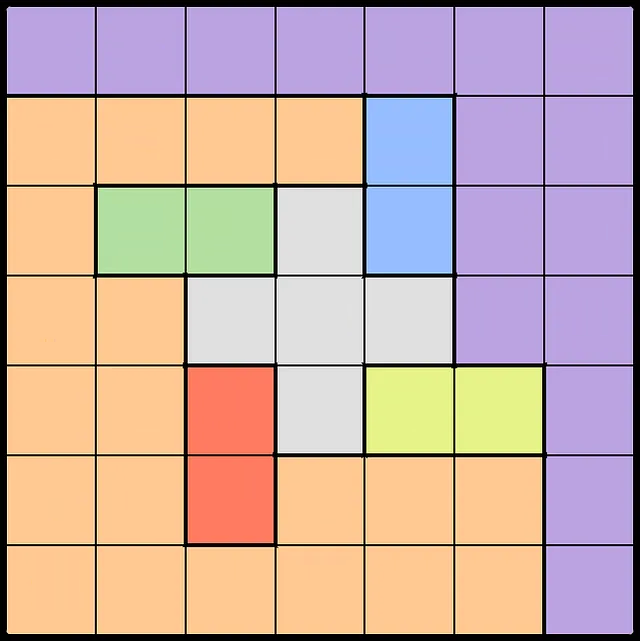
Figure 1:Example of a Queens minigame board. Source: LinkedIn
- Objective
- To place a crown in each row, column, and colored region on the board.
- Rules
- There can only be one crown in each row, column and colored region.
- There cannot be adjacent crowns, not even along adjacent diagonals.
Problem Modeling
Before solving Queens, it is necessary to translate the game elements into the following components of the LOP:
Ranges
Sets
Decision Variables
Objective Function
Constraints
Ranges
Defining the ranges is a fundamental step for the proper definition of the other components of the LOP. For the case of Queens, three ranges will be considered:
- Range of rows, where is the total number of rows on the board (in this case, = 7)
- Range of columns, where is the total number of columns on the board (also = 7 for this case)
- Range of colored regions in game, where is the total number of regions on the board ( = 7)
Sets
By defining the ranges and , let’s define three sets for solving the Queens game:
- Set of all squares on the board, which is nothing more than the Cartesian product of the ranges and
- Set of colored regions and says to which region a square belongs. Each region will be a subset of , composed of the set of ordered pairs that belong to color . Furthermore, the set must be a partition of the set of squares , that is, the union of all its subsets are jointly exhaustive and mutually exclusive, since each square belongs to one color and there is no square that belongs to two different colors.
- Set of all pairs of diagonally adjacent squares. This set will be useful so to make defining the constraints easier later on.
Decision Variables
The decision variables, whose solution we want to find to solve the LOP, will be binary variables , which assume only two values:
- , if the crown is located in row and column ;
- , otherwise.
Objective Function
The interesting thing about the Queens game is that, since we don"t have an objective function to maximize or minimize, we are not actually dealing with an optimization problem, but rather a feasibility problem, that is, our objective is only to find a feasible solution that meets all the game’s constraints. Because of this, we can define the objective function as maximizing (or minimizing, it doesn"t matter) an arbitrary constant. Thus, the objective function will not depend on the decision variables, so that the model doesn"t seek to optimize it and only worries about meeting the constraints.
Constraints
With the previous elements well defined, we can finally translate Queens" rules into constraints for our BLOP model. Let’s go step by step:
- Binarity Constraints
- The first constraint we need to define right away is that all decision variables in our problem are binary variables, meaning they only accept 0 and 1 as valid values.
- Single-Crown-Per-Row Constraints
- Since each row on the board must have only one crown, the sum of all belonging to a row must equal 1. As there are 7 rows in total, there will be 7 such constraints, one for each row.
- Single-Crown-Per-Column Constraints
- The same logic applies to the columns. Since there are 7 columns on the board, there will be 7 more constraints, one for each column.
- Single-Crown-Per-Region Constraints
- The same logic also applies to the colored regions. For each region of the board, the sum of the belonging to a region must be equal to 1. Since there are 7 regions, there will be 7 more constraints.
- Diagonally-Adjacent-squares Constraints
- Finally, we must not forget the rule that there cannot be adjacent crowns, not even along the diagonals. The cases of vertical and horizontal proximity do not need to be addressed, since the row and column constraints already cover this. Therefore, we only need to worry about imposing constraints for the two diagonal directions in each pair of shared-vertex squares. With the set well defined, this constraint is easily defined as it follows.
Abstract Model
With all components defined, it is possible to model the game of Queens using the following abstract model.
Concrete Model
For the Queens game, which will be discussed in this article, we will have the following instance of the abstract model presented earlier, that is, its concrete model.
S.t.:
- Single-Crown-Per-Row Constraints
- (Row 1)
- (Row 2)
- (Row 3)
- (Row 4)
- (Row 5)
- (Row 6)
- (Row 7)
- Single-Crown-Per-Column Constraints
- (Column 1)
- (Column 2)
- (Column 3)
- (Column 4)
- (Column 5)
- (Column 6)
- (Column 7)
- Single-Crown-Per-Region Constraints
- (Purple Region)
- (Orange Region)
- (Blue Region)
- (Green Region)
- (Gray Region)
- (Red Region)
- (Yellow Region)
- Principal Diagonals Constraints
- Secondary Diagonals Constraints
- Binarity Constraints
Solving with Pyomo and NetworkX
Along this book, it’ll be used the following Python libraries that will enable us to solve the games:
- Pyomo
- Open-source library for modeling optimization problems. Its main advantage is the ability to model problems using set logic, which allows defining a set of variables, parameters, and constraints from the definition of other sets of objects. For example, once one defines the set of ranges , , and , it’s possible to define, e.g., the set of squares, regions and diagonals with just one line of code each instead of defining them one by one, saving considerable time!
- NetworkX
- Geared towards manipulating and studying network structures. With it, it’s possible to create graphs and solve problems modeled in network logic quickly and easily, such as the Shortest Path problem, Minimum Spanning Tree, Transportation and Transshipment problem, and other graph problems. Furthermore, it’s possible to quickly draw graphs when combined with Matplotlib.
After installing the solver, let’s import the used libraries.
import matplotlib.pyplot as plt # For displaying the solved game.
import networkx as nx
import pyomo.environ as pyo
Solving Queens
As an example of applying the presented model, the Queens No. 307 problem, published on the platform on March 3rd, 2025, was used.
In order to model and solve the game, it was defined the solve_queen() function in the code below.
def solve_queens(n:int, m:int, regions:dict) -> None:

    # Instantiating the model
    model = pyo.ConcreteModel()

    # Ranges
    I = model.I = pyo.RangeSet(n)
    J = model.J = pyo.RangeSet(m)
    K = model.Colors = pyo.Set(initialize=regions.keys())

    # Sets
    H = model.Squares = pyo.Set(initialize=lambda model: [(i,j) for i in I for j in J])
    R = model.Regions = pyo.Set(K, initialize=regions, dimen=2)
    D = model.Diagonals = pyo.Set(initialize=lambda model: [
        ((i, j), (i+1, j+1)) for (i,j) in H if (i+1,j+1) in H] + [
        ((i, j), (i+1, j-1)) for (i,j) in H if (i+1,j-1) in H
    ])

    # Objective function
    model.obj = pyo.Objective(expr=0, sense=pyo.maximize)

    # Decision Variables
    x = model.x = pyo.Var(H, within=pyo.Binary, initialize=0)

    # Constraints
    model.single_crown_per_row_constraints = pyo.Constraint(
        I,
        rule=lambda model, i: sum(x[i,j] for j in J) == 1
    )

    model.single_crown_per_column_constraints = pyo.Constraint(
        J,
        rule=lambda model, j: sum(x[i,j] for i in I) == 1
    )

    model.single_crown_per_region_constraints = pyo.Constraint(
        K,
        rule=lambda model, k: sum(x[i,j] for (i,j) in R[k]) == 1
    )

    model.adjacent_squares_by_vertex_constraints = pyo.Constraint(
        D,
        rule=lambda model, i, j, r, s: x[i,j] + x[r,s] <= 1
    )

    # Optmization result
    solver = pyo.SolverFactory("gurobi")
    results = solver.solve(model)
    solution = [(i, j) for i in I for j in J if model.x[i,j].value == 1]

    if str(results.Solver.status) == "ok":
        G = nx.grid_2d_graph(n,m)
        plt.figure(figsize=(3.4, 3.4))

        squares = sorted(list(H))
        squares = [(i-1, j-1) for (i,j) in squares]

        color_map = [{(i-1, j-1): region for (i,j) in squares} for region, squares in regions.items()]
        color_map = {square: region for d in color_map for square, region in d.items()}
        color_map = [color_map[square] for square in squares]

        hex_map = {
            "purple": "#BBA3E1",
            "orange": "#FFC794",
            "blue": "#94BEFF",
            "green": "#B3DF9E",
            "gray": "#E0E0E0",
            "red": "#FF7B61",
            "yellow": "#E6F388"
        }

        color_map = [hex_map[color] for color in color_map]

        nx.draw(
            G,
            pos= {(i,j): (j, -i) for i, j in G.nodes()},
            with_labels= True,
            labels= {(i-1, j-1): "O" for (i,j) in solution},
            node_size= 1000,
            node_color= color_map,
            node_shape="s",
            width=0
        )
        plt.show()

    else:
        print("No valid solution was found!")
With the function created, it’s only needed to pass the necessary inputs to solve the Queens game.
regions = {
    "purple": [(1,1), (1,2), (1,3), (1,4), (1,5), (1,6), (1,7), (2,6), (2,7), (3,6), (3,7), (4,6), (4,7), (5,7), (6,7), (7,7)],
    "orange": [(2,1), (2,2), (2,3), (2,4), (3,1), (4,1), (4,2), (5,1), (5,2), (6,1), (6,2), (6,4), (6,5), (6,6), (7,1), (7,2), (7,3), (7,4), (7,5), (7,6)],
    "blue": [(2,5), (3,5)],
    "green": [(3,2), (3,3)],
    "gray": [(3,4), (4,3), (4,4), (4,5), (5,4)],
    "red": [(5,3), (6,3)],
    "yellow": [(5,5), (5,6)]
}

solve_queens(7,7,regions)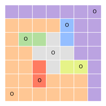
The output board matches the solution of the Queens No. 307, as expected.
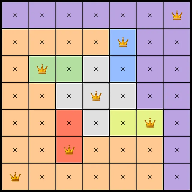
Figure 3:Solution of Queens No. 307, March 3rd, 2025. Source: LinkedIn
References
Queens. LinkedIn. Available at https://
www .linkedin .com /games /queens/. Accessed on Marh 3rd, 2025. BELFIORE, Patrícia; FÁVERO, Luiz Paulo. Pesquisa Operacional: Para cursos de Administração, Contabilidade e Economia. Elsevier Editora Ltda., 2012.
Pyomo. Available at https://
www .pyomo .org/. Accessed on Marh 3rd, 2025. Gurobipy. Gurobi Optimization. Available at https://
www .gurobi .com /faqs /gurobipy/. Accessed on Marh 3rd, 2025. gurobipy 12.0.3. PyPI. July 15th, 2025. Available at https://
pypi .org /project /gurobipy/. Accessed on Marh 3rd, 2025. NetworkX. Available at https://
networkx .org/. Accessed on Marh 3rd, 2025.